Tensor Chain Contraction with Refolds
You can find the source code for this post here.
In a previous post we utilized recursion schemes in prototyping a genetic algorithms library. I wanted to look more into their use cases and was happy to discover that they could even be leveraged for dynamic programming.
Matrix Chain Multiplication
One of my favorite applications of dynamic programming is matrix chain multiplication; given a bunch of matrices with shared indices, the goal is to find the smallest number of arithmetic operations possible in calculating their product. Usually, this is accompanied by deriving the optimal parenthesization.
There are lots of examples online that outline the conventional dynamic programming approach, so I’m not going to rehash it here. I do, however, recommend familiarizing yourself with the dynamic programming solution before moving on. Here, we’ll focus on leveraging recursion schemes to get the job done.
To find the optimal parenthesization, Hinze and Wu leverage a recursion scheme called a dynamorphism, which can be modeled in part with a recursion scheme touched upon in the last post called a hylomorphism, described as a function that unfolds (builds) some intermediate structure (using a CoAlgebra) and folds (reduces) that intermediate structure into some accumulated value (using an Algebra):
type Algebra f a = f a -> a
type CoAlgebra f a = a -> f a

hylo :: Functor f => CoAlgebra f a -> Algebra f b -> a -> b
hylo f g = h where h = g . fmap h . f
Due to this unfolding and folding mechanism, hylomorphisms are sometimes referred to as a kind of refold.
Dynamorphisms, another type of refold, are very similar to a hylomorphism; a dynamorphism performs the same behavior as a hylomorphism but maintains a record of its folds by storing the result of each one into a structure called a Cofree Comonad:
data Cofree f a = a :< (f (Cofree f a))If this looks confusing, don’t fret. It’s extremely similar to a recursive definition of a list type, and we’ll be treating it as such:
-- normal list type
data List valueType =
    Cons valueType (List valueType) | Nil

-- closer to Cofree
data ListS containerType valueType =
    ConsS valueType (ListS containerType valueType)

-- even closer to Cofree
data ListCF containerType valueType =
    ConsCF valueType (containerType (ListCF containerType valueType))

-- basically Cofree
data ListCF containerType valueType =
    valueType :< (containerType (ListCF containerType valueType))
Let’s compare the signature of a dynamorphism to a hylomorphism without the type synonyms:
hylo :: Functor f => (a -> f a) -> (f b -> b)            -> a -> b
dyna :: Functor f => (a -> f a) -> (f (Cofree f b) -> b) -> a -> b
We can see that they are pretty similar, and we can see in the definition of dyna that this really is a hylomorphism that keeps track of the values calculated:
-- extracts the first value from Cofree
extract :: Cofree f a -> a
extract (a :< _) = a

dyna :: Functor f => (a -> f a) -> (f (Cofree f b) -> b) -> a -> b
dyna h g = extract . hylo h (\fcfb -> (g fcfb) :< fcfb)
The dynamorphism builds an intermediate structure with h a and it stores the result of applying g to that value in a Cofree. Using our list analogy, it’s applying g to the incoming functor and prepending the result to an existing list of past-calculated values. This is reminiscent of the iterate function, which repeatedly applies a function f to some value x and appends each application’s result to a list.
By keeping a history of the dynamorphism’s applications of the folding function it’s supplied, one can reach back into the Cofree structure and utilize pre-calculated values a la dynamic programming, which is exactly what Hinze and Wu do for matrix chain multiplication:
-- grab the nth element of a Cofree
get :: Cofree (ListF v) a -> Int -> a
get (x :< xs) 0 = x
get (x :< (Cons _ xs)) n = xs `get` (n-1)

-- take the first n elements of a Cofree
collect :: Cofree (ListF v) a -> Int -> [a]
collect _ 0 = []
collect (x :< (Some _)) n = [x]
collect (x :< (Cons _ cf)) n = x : cf `collect` (n-1)

chainM :: [Int] -> Int
chainM dims = dyna triangle findParen range where

    range = (1, length dims - 1)

    triangle :: (Int,Int) -> ListF (Int,Int) (Int,Int)
    triangle (1,1) = Some (1,1)
    triangle (i,j)
        | i == j = Cons (i,j) (1,j-1)
        | otherwise = Cons (i,j) (i+1,j)

    findParen :: ListF (Int,Int) (Cofree (ListF (Int,Int)) Int) -> Int
    findParen (Some j) = 0
    findParen (Cons (i,j) table)
        | i == j = 0
        | i < j = minimum (zipWith (+) as bs) where
            as = [(dims !! (i-1)) * (dims !! k) * (dims !! j)
                   + (table `get` offset k) | k <- [i..j-1]]
            bs = table `collect` (j-i)
            offset k = ((j*(j+1) - k*(k+1)) `div` 2) - 1
With dependencies between subproblems modeled as a directed acyclic graph, the algorithm unfolds a range into a list of cell coordinates in reverse topological order using the triangle function. It then folds that list in topological order with findParen, maintaining a table of past-calculated values along the way. With every folding step, findParen reaches back into the table to find the pre-calculated values in cells (i,k) and (k+1,j) for every k in the range [i,j-1] and finds the best k to split the intermediate matrix Mij. As you can tell from the way these values are calculated, Hinze and Wu carefully consider and identify where these previously-calculated values may be found in the Cofree.
However, there are two pieces causing this function to lose the 𝒪(N3) complexity found in the conventional dynamic programming approach; our first problem is that Haskell lists are not built like typical arrays, but like linked lists, so dims !! x has complexity 𝒪(N) rather than the desired 𝒪(1) – but this at least can be remedied with something like Data.Vector. Our second problem is similar; Cofree is like a linked list, and so reaching into the Cofree structure with get is a linear operation; the pre-calculated value at offset k is not guaranteed to be within a constant distance of the head of Cofree. If we were calculating something like the nth Fibonacci number, we would only need to look back two elements and would be in the clear, but here it is not the case; we’ve caused the overall complexity to reach 𝒪(N4).
I’m unaware of a way that something like Cofree can allow us to peek into its structure in constant time, particularly when the element we’d like grab is arbitrarily nested. So, instead of relying upon a dynamorphism, we can return to a hylomorphism – and, instead of a list or a vector of pre-calculated scores with nontrivial offset calculations, we’ll maintain a “two-dimensional” memoization table. For simplicity’s sake, we’ll leverage a HashMap, but one could easily use Data.Vector. So, findParen will then take the following form:
type Map = HashMap.Map

chainM :: [Int] -> Int
chainM dims = best where
    best = (hylo triangle findParen range) ! range

-- ...

    findParen :: Algebra (ListF (Int,Int)) (Map (Int,Int) Int)
    findParen (Some (j,_)) = Map.insert (j,j) 0 Map.empty
    findParen (Cons (i,j) table)
        | i == j = Map.insert (i,j) 0 table
        | i < j = Map.insert (i,j) (minimum parenthesizations) table where
            cost x y = table ! (x,y)
            space (x,y,z) = (dims !! x) * (dims !! y) * (dims !! z)
            parenthesizations =
                [space (i-1,k,j) + cost i k + cost (k+1) j | k <- [i..j-1]]
With this change and an imagined switch to Data.Vector for the sequence of dims, we can bring the time complexity back to 𝒪(N3)*.
* Sort of, the unordered-containers package mentions “[m]any operations have a average-case complexity of 𝒪(logN). The implementation uses a large base (i.e. 16) so in practice these operations are constant time.” If we really wanted constant time, we could use a two dimensional Vector but we’ll stick with HashMap for simplicity.
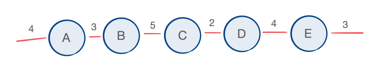
For a chain of matrices such as:

we can see the minimum number of operations possible is 102:
let matrices = [4,3,5,2,4,3]
putStrLn . show $ chainM matrices -- 102
Tensor Chain Contraction
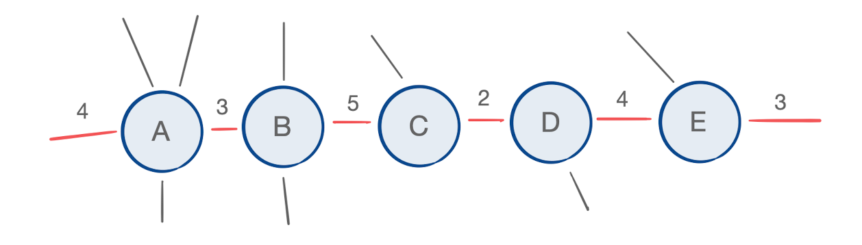
We can view this chain of matrices as a graph with weighted edges that we’d like to contract together; each matrix multiplication costs the product of all edge weights incident to the matrices being multiplied, up to a constant factor:
If the relationship between the equation and diagram is escaping you, I encourage you to check out the wonderful tutorial by Tai-Danae Bradley, which indicates that matrix multiplication is a special case of tensor contraction. Let’s take a look at a different graph:
Instead of matrices with two dimensions, we have multidimensional tensors with some indices that are free. The problem is now to find the optimal parenthesization of a chain of tensors to be contracted.
Additionally, the indices of the tensors involved in the chain contraction need not be free; they can be bound to other tensors outside of the chain of interest, or even to other tensors in the chain.
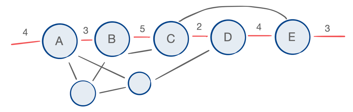
We can now put our sights on finding the optimal contraction order of a path within some arbitrary tensor network.
It turns out that we can apply the same dynamic programming approach to tensor chain contraction – and credit goes to my colleague Jonathan Jakes-Schauer for the insight. The key is to keep track of all indices that are incident to the chain of interest, because they’ll each contribute to the cost of the contractions in which their tensors participate.
For matrix chain products we saw that findParen identified an index k that optimally decomposed a given intermediate matrix into two. This calculation recursively depended upon the optimal way to decompose those two matrices, down to the original matrices in the chain (which cost nothing to construct). The question then is how to calculate the cost of contracting two tensors; two contracted tensors may share more than just one index, and so we must account for more than just the dimensions of those indices, as we did before. To illustrate, consider the example below:
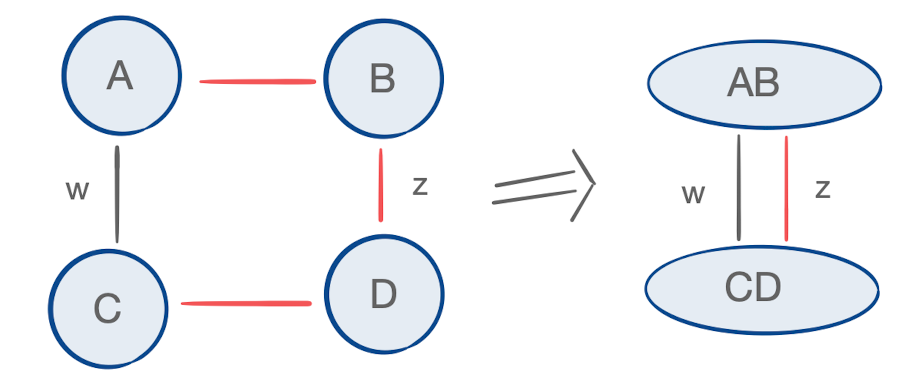
Once tensor A has been contracted into B, and C into D, the resulting intermediate tensors AB and CD share two indices. Because index w was originally incident to neither tensor B nor D, it’s important that we don’t overcount the number of operations associated with contracting AB and CD; if this contraction appeared in the dynamic programming routine with i = 1, k = 2, and j = 4, and we calculated the cost as before without regard to the identity of the indices involved, we would cost this contraction at wzw rather than the true cost, which is wz. Towards this end, we’ll maintain the identity of all indices participant to and resulting from each contraction, using the following types:
type Tensor = Map Int Int

data ContractionTree a =
    Tensor a
  | Intermediate (ContractionTree a) (ContractionTree a)


data TensorData = TensorData {
    totalCost :: Int,
    recipe :: ContractionTree Int,
    indices :: Tensor
}
where totalCost denotes the cost of the contraction plus the total cost of having created each of the two tensors being contracted, recipe is a helper datatype for knowing the order in which those two tensors were created and contracted together, and indices is the resulting tensor itself, represented by the bundle of incident indices – a mapping from index identifiers to their dimensions.
Suppose we would like to contract two tensors and want to know the resulting totalCost and indices using a function with the following type:
contract :: (TensorData, TensorData) -> TensorDataSuppose the indices of those two tensors are a given and we’d like to know what indices are left over from the contraction. We can see from an example like the one below:
that the indices left over from the contraction are equal to the symmetric difference of all indices incident to the tensors being contracted:
contract :: (TensorData, TensorData) -> TensorData
contract (left,right) = TensorData {
    totalCost = ...,
    recipe = ...,
    indices = symDiff (indices left) (indices right),

} where
    symDiff l r = (l \\ r) <> (r \\ l)
where x \\ y is the set difference, or x - y, and x <> y is the set union.
We’ve mentioned already that the cost of contracting two tensors is the product of all indices incident to the two tensors. More formally, for tensors A and B, the cost of contraction is

where I(X) denotes the set of indices belonging to some tensor X. Given this, and set of indices we’ve maintained from earlier contractions, we can then calculate the cost of splitting an intermediate tensor as was done in the case of matrices. We identify two “child” tensors when splitting some intermediate tensor as discussed above; it’s determined by the start i of the subchain in question, the end j of the subchain in question, and the marker k, where the chain shall be split; the intermediate tensor TiTi + 1..Tk = Tik marks the first tensor, and Tk + 1Tk + 2..Tj = T(k+1)j marks the second. When contracted, they result in tensor Tij.

With this, we have all the information necessary to represent the resulting tensor:
tspace = Map.foldl (*) 1

contract :: (TensorData, TensorData) -> TensorData
contract (left,right) = TensorData {
    totalCost = tspace (indices left <> indices right)
                + (totalCost left)
                + (totalCost right),
    recipe = Intermediate (recipe left) (recipe right)
    indices = symDiff (indices left) (indices right),

} where
    symDiff l r = (l \\ r) <> (r \\ l) -- symmetric difference
However, calculating the symmetric difference as well as the union of the indices incident to participant tensors is 𝒪(R), where R is maximum order among tensors contracted. If we do this for every Tik and T(k+1)j, we’ve increased the complexity of our algorithm to 𝒪(RN3).
Can we do better? Can we calculate cost and symmetric difference in a way that’s independent of k to store in our memoization table for when it’s time to consider Tij?
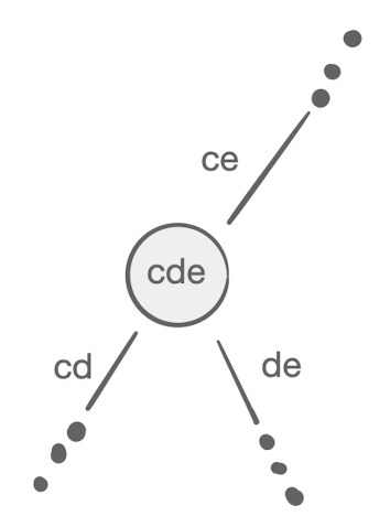
Let’s consider the symmetric difference, which is associative. If we have an intermediate tensor Tij, no matter which value for k we evaluate, the set of indices belonging to Tij will always be the same. So, we don’t need to calculate this for every value of k after all, we only need to reach into the memoization table to find one k value that’s already been considered. Where can we find that k? If we look back at the triangle function, we receive a hint:
    triangle :: (Int,Int) -> ListF (Int,Int) (Int,Int)
    triangle (1,1) = Some (1,1)
    triangle (i,j)
        | i == j = Cons (i,j) (1,j-1)
        | otherwise = Cons (i,j) (i+1,j)
for a given pair (i,j), we append that pair to a list containing (i+1,j) at the head. So, by the time we reach (i,j) in our fold within findParen, (i+1,j) is already in the memoization table. This means that a value k = i has already been accounted for and we can access the information for Tii and T(i+1)j, and calculate the symmetric difference, i.e. the indices leftover from the contraction:
indLeft = indices $ table ! (i,i)
indNext = indices $ table ! (i+1,j)
symdiff = (indLeft \\ indNext) <> (indNext \\ indLeft) -- O(R)
That’s one half of our problem solved. Unfortunately, the same intuition cannot be applied to finding each contraction cost, which is not associative. This is obvious when you consider for a moment that, if it were, this problem of finding the optimal parenthesization wouldn’t exist!
This doesn’t completely kill our chances of remaining independent of k, however, it just means we can’t do so and continue thinking about cost in the same way. So, let’s think about it another way.
Contraction Trees
Described in Carving-width and contraction trees for tensor networks, a contraction tree is a data structure describing a particular set of tensor contraction orders. For example, take a look at the following parenthesization of our matrix chain and notice its mapping to a contraction tree:
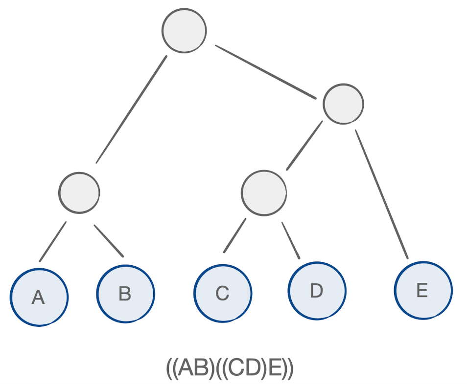
If this chain was comprised of higher-order tensors, the concept would remain the same.
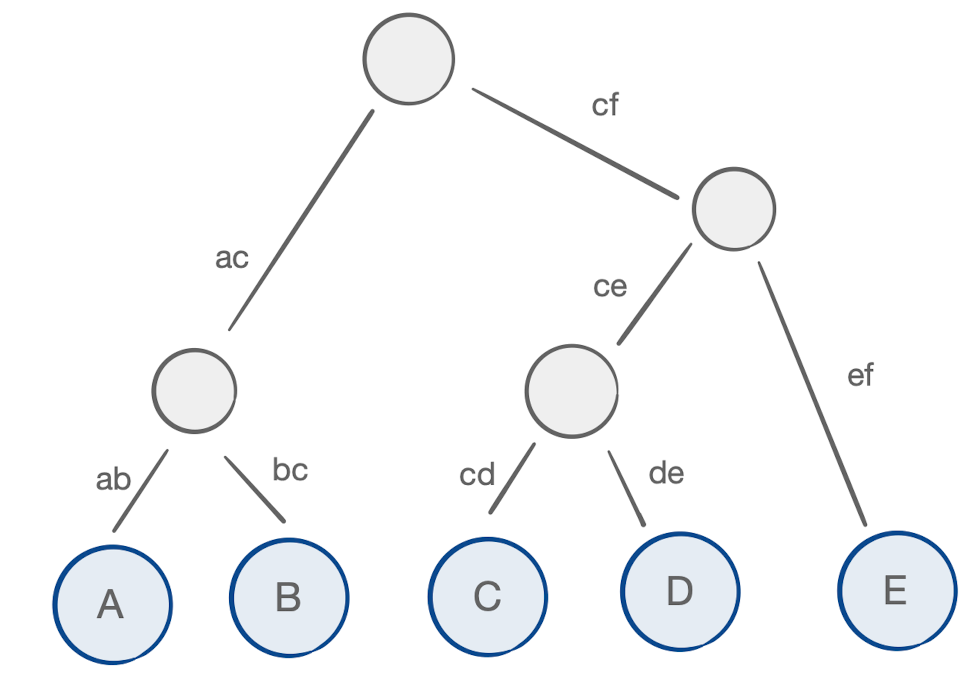
We can weight the arcs of this tree, where the weight corresponds to the symmetric difference of the indices incident to the tensors getting contracted. We start with the arcs incident to the leaf nodes, corresponding to the original tensors and their indices:
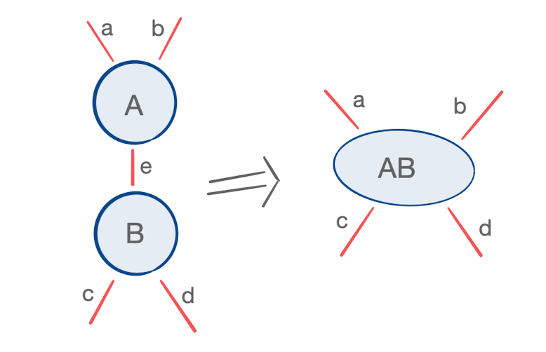
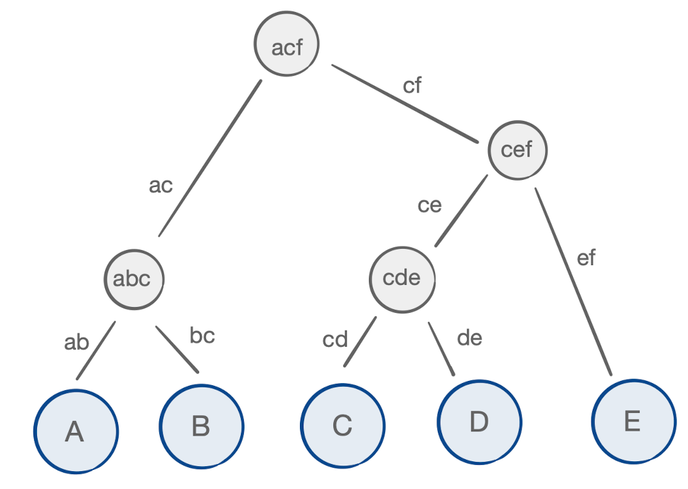
Similarly, we can weight each internal node, representing each intermediate tensor, with their cost of creation – the product of the set union of its protruding arcs:
If you look closely at each internal node, you’ll notice one interesting property:
For each node with arcs a, a′, and a″, the weight of the node itself, i.e. the cost of its creation, is:

We can reconsider the labels of our arcs in a way that captures the nature of the problem at hand:

With this we can see that the weights of arcs correspond to the set of indices child tensors Tik and T(k+1)j and their result, Tij, each contain. By maintaining an account of those arc weights, we can calculate the cost of the contraction in a way that relies on the associative symmetric difference. In other words, we can now calculate the cost in a way that’s independent of k. First, we’ll add a new attribute called cspace that captures this arc weight:
data TensorData = TensorData {
    totalCost :: Int,
    recipe :: ContractionTree Int,
    cspace :: Int,
    indices :: Tensor
}
which we can utilize in calculating the cost:
    indLeft = indices $ table ! (i,i)
    indNext = indices $ table ! (i+1,j)
    symdiff = (indLeft \\ indNext) <> (indNext \\ indLeft) -- O(R)
    cspaceij = tspace symdiff -- O(R)

    -- get contraction data of combining two intermediate tensors: O(1)
    contract :: (TensorData, TensorData) -> TensorData
    contract (left,right) = TensorData {
        totalCost = totalCost left + totalCost right + sqrtCspaces,
        recipe = Intermediate (recipe left) (recipe right),
        cspace = cspaceij,
        indices = symdiff
    } where
        cspaces = cspace left * cspace right * cspaceij
        sqrtCspaces = round . sqrt . fromIntegral $ cspaces
Wrapping Up
Putting everything together, we now have everything we need for an algorithm that can calculate the tensor chain product for any path in a tensor network in 𝒪(RN2+N3) time. After addressing the portions of our memoization table that correspond to our original tensors, we have our final result:
chainT :: Vector Tensor -> TensorData
chainT tensors = best where

    best = (hylo triangle findParen range) ! range
    range = (1, length tensors)

    emptyData i = TensorData {
        totalCost = 0,
        recipe = Tensor i,
        cspace = tspace t,
        indices = t
    } where t = (V.!) tensors (i-1)

    triangle :: (Int,Int) -> ListF (Int,Int) (Int,Int)
    triangle (1,1) = Some (1,1)
    triangle (i,j)
        | i == j = Cons (i,j) (1,j-1)
        | otherwise = Cons (i,j) (i+1,j)

    findParen :: Algebra (ListF (Int,Int)) (Map (Int,Int) TensorData)
    findParen (Some (t,_)) = Map.insert (t,t) (emptyData t) Map.empty -- O(R)
    findParen (Cons (i,j) table) -- O(R + N) per (i,j)
        | i == j = Map.insert (i,j) (emptyData i) table -- O(R)
        | i < j = Map.insert (i,j) best table where

            -- O(R)
            indLeft = indices $ table ! (i,i)
            indNext = indices $ table ! (i+1,j)
            symdiff = (indLeft \\ indNext) <> (indNext \\ indLeft)
            cspaceij = tspace symdiff

            -- O(N)
            splits = [((i,k),(k+1,j)) | k <- [i..j-1]]
            getData (l,r) = (table ! l, table ! r)
            parenthesizations = map (contract . getData) splits
            best = argmin totalCost parenthesizations

            -- O(1)
            -- get contraction data of combining two intermediate tensors
            contract :: (TensorData, TensorData) -> TensorData
            contract (left,right) = TensorData {
                totalCost = totalCost left + totalCost right + sqrtCspaces,
                recipe = Intermediate (recipe left) (recipe right),
                cspace = cspaceij,
                indices = symdiff
            } where
                cspaces = cspace left * cspace right * cspaceij
                sqrtCspaces = round . sqrt . fromIntegral $ cspaces
As a sanity check, we can evaluate the same matrix chain we started with:
main = do
    let tensors = V.fromList $ map (Map.fromList) [
                [(1,4),(2,3)],
                [(2,3),(3,5)],
                [(3,5),(4,2)],
                [(4,2),(5,4)],
                [(5,4),(6,3)],
                [(6,3),(7,2)]
            ]

        matrices = [4,3,5,2,4,3,2]

    putStrLn . show . chainM $ matrices -- 102
    putStrLn . show . totalCost . chainT $ tensors -- 102